In an earlier blog we traced the development of transformer from NLP evolution in the historical perspective. Inspired by the concept of self-attention, information theory and signal processing, transformer became the building block of well-known LLMs developed by OpenAI, Google and Meta. The simplicity of transformer intuition and its adaptability for efficient parallel computing have rendered it to be extremely useful. This enabled them to surpass the limitations of earlier recurrent neural network or convolution neural network of deep neural networks. It will be enlightening to look at transformers from signal processing and information theory concepts as to how these ideas combined with deep neural networks created the modern marvel called “transformer”. We will then review some of the later LLM developments based on transformers
We first discuss encoders and decoders for NLP, an idea taken from signal processing principles. Formulating the RNN and its improved variants using this framework helps in clear understanding of principles as well as several use cases. This will give an entirely new turn to the idea of seq2seq processing. Having set this background, we will start to look from an information theory point of view at the structure of processing needed for resolving NLP prediction problem. This naturally leads to the concept of perplexity and how deep neural networks can help to decrease the perplexity for NLP tasks. Then follows a discussion of transformer architecture and its usage variants. We finally wrap up with some discussion of well-known LLMs that are built based on transformers.
Encoders and Decoders
In signal processing, the concepts of encoders and decoders are foundational for transforming and interpreting signals, and their relevance extends deeply into modern transformer architectures. In fact, this encoder-decoder framework is central to the success of the LLMs, which are in turn a significant milestone in NLP and enabled breakthrough in NLP tasks. An encoder transforms an input signal into a new representation, often compressing or reshaping the data to highlight the most meaningful features. This transformation allows for the extraction of essential information that can be processed more efficiently or effectively. In particular, for transformers, the encoder operates similarly by converting input data into a series of context-aware embeddings. These embeddings capture both local and global relationships within the data, enabling the model to represent complex patterns. This step is crucial in creating a compact, high-quality representation that facilitates later stages of processing.
A decoder in signal processing takes the transformed signal and reconstructs it, ideally recovering the original or extracting desired insights. Decoders interpret encoded information to make it comprehensible, akin to translating compressed or encrypted data back into human-readable form. In particular for transformers, the decoder takes the encoded embeddings and transforms them into an output sequence, which can be text, audio, or another form of structured data. The decoder leverages information from the encoder to accurately generate coherent outputs, often using attention mechanisms to focus on relevant parts of the encoded input.
ANN and CNN are not well-suited to handle sequential data such as time-series or genome or financial or textual data. For example, for machine translation tasks, where both the input and output are sequential, ANN and CNN models struggle with the complexities of alignment of variable input and output sequence lengths. Recurrent Neural Networks (RNNs) are a class of neural networks specifically designed for sequential data, where the order of data points matters. Unlike traditional feedforward neural networks, which treat each input independently, RNNs have an internal memory that allows them to retain information about previous inputs, making them ideal for tasks where context or history is crucial, such as language processing, time-series forecasting, and speech recognition. The feedback mechanism enables RNNs to retain information from previous inputs (past time steps), giving them a sort of “memory” for context. There RNNs are further improved as Long Short-Term Memory (LSTM)networks and Gated Recurrent Units (GRU) networks,
The encoder-decoder architecture is a core framework for handling sequence-to-sequence (Seq2Seq) problems, where the goal is to transform one sequence (input) into another (output) of potentially different length and structure. Seq2Seq tasks often involve sequences of variable lengths, such as translating sentences, summarizing documents, or converting audio into text. Various sequences from left to right and their use cases are described below:
(1) One-to-One: Fixed-sized input to fixed-sized output (e.g. Image Classification).
(2) One-to-Many: Sequence output (e.g. Image captioning).
(3) Many-to-One: Sequence input and fixed-size output (e.g. sentiment analysis)
(4) Many-to-Many (No sync): Sequence input and sequence output (e.g. Machine Translation).
(5) Many-to-Many (Sync) : Synced sequence input and output (e.g. Video Classification where we wish to label each frame of the video).
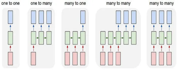
The encoder-decoder architecture as shown in Figure 1 is well-suited to this, as the encoder compresses the input sequence into a meaningful representation that the decoder can then expand into the target sequence. The encoder creates a “context” or “embedding” for the input, which is a fixed-size representation regardless of the input length. This encoding contains the core information needed by the decoder to reconstruct the output sequence.
The encoder processes the input sequence, capturing both local and long-range dependencies within it. This is essential for Seq2Seq tasks because each part of the input sequence might be relevant to various parts of the output sequence. For example, in machine translation, certain words in a sentence can affect the meaning of words much later in the output sentence. The encoder processes the information into fixed-length context vector, which captures the essence of the input data, summarizing its information content. By building a context-rich representation, the encoder provides the decoder with an informative starting point, even for complex sequences.
The decoder generates the output sequence step-by-step, informed by the encoder’s representation and often by prior output tokens (in an autoregressive manner). This is especially useful for generating coherent and contextually relevant output, such as translating “The weather is nice” in English to “Le temps est agréable” in French. During each step, the decoder predicts the next token based on the encoder’s information and its own output history, making the architecture powerful for tasks where output depends on previous predictions (e.g., language generation).
While processing NLP, it is necessary to introduce a new way of word embeddings, such as Word2Vec, GloVe, and FastText. These are dense, low-dimensional vector representations of words to capture semantic and syntactic relationships. In Word2Vec, NNs generate embeddings by optimizing a model to predict nearby words in a text. In contrast, traditional n-grams and HMM struggle with representation of long-term dependencies.
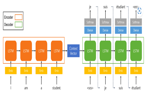
The encoder part is an LSTM cell. It is fed in the input sequence over time, and it tries to encapsulate all its information and store it in its final internal states hₜ (hidden state)and cₜ (cell state). The internal states (‘context vector’) are then passed onto the decoder part, which it will use to try to produce the target sequence. Given the input sequence X = {x1, x2, …, xT} and the encoder’s initial hidden state h0 initialized to
zero. The computation of hidden state is updated as ht = fenc (ht-1, xt) for t=1 to T and the context vector is finally computed as hT. The decoder’s initial hidden state “s0” is set to the context vector hT. The computation of the output state is st = fdec (st-1, yt-1), where st is decoder’s hidden state at time t, fdec is decoder’s activation function. The output is calculated as p (yt | y<t, X) = SoftMax (Wst) where W is the weight matrix for the output layer and p(yt | y<t , X) is probability distribution over the possible outputs at time t.
The main challenges to RNN are during training phase. Backpropagation through time (BPTT) is used to calculate gradients over several time steps. Therefore, for long sequences, gradients can become extremely small (vanishing) or extremely large (exploding), making it difficult for RNNs to learn long-range dependencies effectively. A general rule of thumb is that the deeper a neural network is, harder it is to train. The improved versions, LSTN and GRU, help mitigate issues like vanishing gradients to a limited extent. In addition, the mainultimate hidden state of LSTM is tasked with encapsulating the entire sentence for translation. This will typically be only a few hundred units (i.e., floating-point numbers). Therefore, too much cramming increases showiness in the DNN output
Perplexity Approach Next Word Prediction
A language model of a document is a probabilistic model p(x1, x2, … xT; Θ) where Θ is the parameter, T is the number of tokens and V is the dictionary size. This produces a distribution over V different choices and using probabilities identities the p(.) can be expressed as conditional probabilities in the following way:
p(x1, x2, … xT) = ΠTt=1 p(xt | x1, x2, … xt-1)
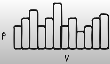
We will be using autoregressive model to predict the next token conditioned on previous tokens. This produces probability histogram distribution over all possible V choices as shown in Figure 2.
Another interesting thing about joint distribution is that we can sample a document by sampling each of the words individually one at a time, feeding it as the conditional to the next step and then sampling the next word. We can sample x1 first and use it in the conditional in the next step to sample x2, then x3 and so on until we sample xT. It was very common until recently to assume that the probability of xT really only depended on a few of the previous words for instance we might assume that xT only depends on xT-1. It is indeed true that definitely xT-1 provides the more information about predicting xT than the words that are further away. Another assumption is that the probability of the next word could be modeled with one step categorical distribution model. As language modelling is unsupervised learning it’s hard to quantify when a model is good or when it’s bad. One way is to give it unseen text and then check how close its predictions are to the predictions in that text.
Suppose given a sentence “The dog walk to the” we might want to accurately predict the next word and measure the metric. Suppose the categorical model predicts “park” whereas the true answer is “lawn.” The alternative is syntactically correct although it is factually wrong and with accuracy metric we get zero score. Further, given the nature of natural English language which follow Zipf distribution, things get complicated. As per Zipfian distribution, familiar words make up a large portion of the probability mass, but very uncommon words are seen pretty frequently. This means the common word like “the” can easily be predicted but it will be particularly challenging to predict uncommon words like pizza or raincoat, which may have more or less same probability. What this means is that a lot of the time we are going to predict pretty simple words like “the” correctly but not too infrequently will fail to predict the exact word accurately. If we efficiently source code the words of language model with probability distribution “p”, we can show that the average bits needed is upper bounded by 1/T ∑t -log2(p (xt | x1, x2, … xt-1)). This is alternatively referred to as entropy of the language model. For historical reasons, the metric, called “perplexity” which is power 2 raised to entropy turned out to be a good one. This allows for comparison of different language models rather than just. checking accuracy naively.
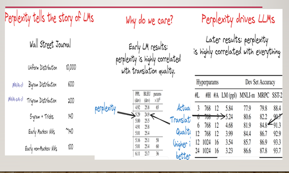
If perplexity is “1” this implies that the number of bits needed per word is zero, then it is deterministic, and we actually don’t need to communicate anything. If the perplexity is 10,000 this implies the distribution is uniform and that we need a string of size log2(10,000) to communicate any word in the dictionary. In general, a uniform probability distribution p with exactly k outcomes has the perplexity “k”. If PP(A) < PP(B), then the lang model A is better comparted to the lang model B.
The benchmark of language modeling problem is to use “The Wall Street Journal Corpus,” which can be thought of as a couple years of newspaper articles as training data and then trying to assess perplexity on today’s newspaper as shown in Figure 2. If we start with uniform distribution, it is “10000” and reduces with bigram, trigram distribution. Early Markov models got the perplexity to about 140. Developing non- Markoff neural networks that looked at longer ranges they could get down to around “100” or even lower. In 2015, researchers found out that language modeling was a good proxy that could be directly utilized for other NLP tasks. For example, English to French machine translation can be modeled as a conditional language modeling problem. It can be seen that the lower perplexity score is correlated to good translation BLEU scores. Further, researchers found that perplexity on the task of language modeling by itself could be used to produce models that would be really good at NLP tasks. Figure 3 demonstrates an interesting result that as raw language modeling perplexity goes down from 5.84 to 3.23 over a series of experiments at the same time three other very different downstream tasks all get significantly better. Moreover, these tasks were not included as part of the original training data. This crucial idea underlies all modern LLM research.
Motivation for Transformers
Two important modifications are needed to get to LLM. The first one is the use of neural network (NN) model, rather than limited Markovian model and the second is to figure out how to consider all previous words. Moving to NN needed a mechanism to represent the word as vectors of size T. To start with, let us take a Markovian model where output depends on the last 2 words and use NN model to make next word prediction. Here input vectors will be one-hot vectors of size T and NN will process previous tokens and output a vector of size T. The output is transformed into a distribution over our vocabulary of size T by applying the softmax function which ensures that the output is positive and sums to one. The softmax operation involves exponentiating each element of the vector and then normalizing which produces a probability histogram.
Though bag-of-words, one-hot encoding word-to-vector representations were there, word2vec representation, which is proposed in 2015, has word embeddings based on the words’ contexts and other pros that became foundational to later NN models. However, it required better computing infrastructure and hardware, which were not available in 2015. The motivation to include all the previous tokens can be seen as follows. Take the sentence “the dog walk to the park” and if the last two words are used to predict the next word; When we come “to the” part, this tells us that it’s a location and a noun, but it really doesn’t tell us much about the semantics of the sentence. If we somehow know who is going or what the verb was that can help us get the next word right. In general, for good prediction there is a need for long term memory and fully autoregressive models that have the ability to utilize all previous tokens.
Further it helps to look at models that make use of an approach called “attention” that allows us to build fully autoregressive models of relatively long range. The concept of “attention” can be thought of as a neural network version of random-access memory or even simpler as a neural network version of a lookup table. We’re going to save all the previous information and then refer back to it as we need it as per the context of the sentence. To implement the attention mechanism, we need three different pieces of information, the first vector known as the query which has looked at the whole sentence so far and addition a lookup table which has a key and a value for each previous position. Based on the query we will match the key that we think will be most relevant to our next word prediction from that key we’ll then extract the corresponding value that value will then be passed to a neural network which we can utilize to predict the next word.
First match the query to the keys to get a score for each location and then compute a softmax over these key locations which gives us a histogram. Then use histogram to average together the values to produce a new intermediate value. The weighted average of these intermediate values is used to predict the next word. This process is a good way to decide which previous words are useful for the next prediction this attention.
Thus the combination of neural networks with attention lead to well-known transformer architecture. The concept of attention is repeatedly used to predict the next word, and the repetition value is hyperparameter. Transformer architecture has become quite iconic in the field it generally consists of two stages the first stage is the attention, and the second stage is a large standard neural network, and these two stages are repeated many times before the final prediction is made.
In the practical situation Q, K and V represent matrices respectively of query, key and values. The transformer operation is represented as “softmax (QKT)V. Here we can see the first step of query scoring with key and softmax normalizing scores. The final output is weighted by the matrix V. Because of matrix multiplication, computation is efficient and because of attention, several such queries, keys and values combinations can be computed in parallel.
Transformers Architecture
Figure 3 shows a stack of encoders on the left and a stack of decoders on the right. Each encoder and decoder are made up of multiple identical layers, typically six to twelve. The encoder is responsible for capturing the pattern of the original sentence, whereas the decoder is employed to generate the corresponding translation. The encoder transforms the input sequence into a set of encoded representations. First, the input sequence X is embedded into a high-dimensional space. This embedding captures the meaning of each word in the sequence. Positional encodings are added to these embeddings to help the model understand the position of each word in the sequence. Although attention mechanism captures the relationships between words, it does not retain the sequence of the words itself
Multihead Attention block basically works by comparing each word with every other word within the sequence. It acts like a group of experts, each focusing on a different aspect of the input sequence. It splits the input into multiple smaller attention heads. Each head independently projects the input into query, key, and value vectors, calculates attention scores, and combines the results. The outputs from all heads are then concatenated and transformed to produce the final result. This process allows the model to capture various relationships within the input sequence. Following the multi-head attention mechanism, the encoder includes a position-wise fully connected feed-forward neural network. This part consists of two linear transformations with a ReLU activation function in between, operating independently on each position in the sequence. This helps transform the information into a richer representation, adding non-linearity to the model and allowing it to learn complex patterns. This is followed by a residual connection and layer normalization. Residual connections, also known as skip connections, help mitigate the vanishing gradient problem by allowing gradients to flow directly through the network. This is done by adding the input of the sub-layer to its output. Layer normalization then stabilizes and speeds up the training process by normalizing the output of the sub-layer, ensuring that the distribution of values remains consistent. Linear block after the decoder is another standard linear layer.
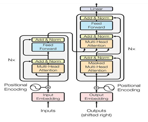
The decoder in a transformer shares several similarities with the encoder but also introduces some key differences to facilitate its role in generating output sequences. Just like the encoder, the decoder is made up of multiple identical layers. Each of these layers contains sub-layers that include multi-head attention and a feed-forward neural network. Both the encoder and decoder use residual connections and layer normalization to enhance learning and maintain stable gradients. The primary difference is the addition of a third sub-layer in each decoder layer, known as the masked multi-head attention mechanism. This extra sub-layer allows the decoder to focus on previously generated tokens while maintaining the autoregressive property of sequence generation. Additionally, the decoder’s multi-head attention mechanisms are designed to handle two sources of information: the input sequence (from the encoder) and the partially generated output sequence.
The masked multi-head attention mechanism is unique to the decoder. It operates similarly to the standard multi-head attention used in the encoder but includes an additional masking step. This masking ensures that the decoder cannot look ahead to future tokens in the sequence during training, preserving the autoregressive nature of the model. During the attention calculation, a mask is applied to the input sequence, setting the attention scores of future tokens to negative infinity. This effectively prevents the model from considering future tokens when generating the current token, ensuring that each token is generated based only on the past tokens and the encoded input sequence.
The decoder’s multi-head attention sub-layers, including the masked multi-head attention and the standard multi-head attention (which attends to the encoder’s output), work together to generate the output sequence. The masked multi-head attention allows the model to generate tokens one at a time, while the standard multi-head attention integrates information from the encoder, enabling the decoder to produce coherent and contextually accurate outputs.
LLMs based on Transformers
The significance of Transformer is aptly captured in the following quote from Andrej Karpathy: “The transformer is magnificent neural network architecture because it is a general-purpose differentiable computer. It is simultaneously: 1) expressive (in the forward pass) 2) optimizable (via backpropagation + gradient descent) 3) efficient (high parallelism compute graph”. We now look at well-known important LLM designs proposed based on the transformer model, training corpus and usage.
BERT (Google, 2019)
Bidirectional Encoder Representations from Transformers (BERT) is an encoder-only architecture developed by Google in 2019. BERT reads text both forward and backward unlike GPT models. Bidirectionality allows BERT to consider the full context of a word by looking at the words before and after it in a sentence, which often improves understanding of the word’s meaning. BERT is pre-trained on a large text corpus like Wikipedia and BooksCorpus but scale and diversity of data are limited compared to LLMs. BERT masked 15% of words randomly and the training objective is to predict these words. In addition, given two sentences, BERT is trained to predict whether the second sentence follows the first one in the original text. This is not a generalist model and required fine-tuning on specific downstream tasks such as classification, named entity recognition etc. BERT is good at NLS tasks but not in general adaptive. BERT comes in various shapes and the number of parameters range from 110 million to 340 million. RoBERTa, DistilBERT and ALBERT are various versions and adaptations of BERT
Text-To-Text Transfer Transformer(T5) (Google, 2019)
T5 is based on encoder and decoder architecture where both input and output are text strings. It builds upon advancements in transformer-based models like BERT and GPT but introduces several key innovations, particularly in framing all NLP tasks as a text-to-text problem. T5 is pre-trained using a task called span corruption, where a portion of the input text is randomly masked, and the model is trained to predict the missing text spans. T5 uses Colossal Clean Crawled Corpus (C4) dataset that’s a cleaned-up version of Common Crawl’s web crawl corpus. The latter has over 50 TB of compressed data and over 10 billion web pages. This is cleaned up applying simple heuristic filtering and deduplication. Finally, the training set is filtered down to 800 GB or about 160 billion tokens.
The advantage of T5’s unified text-to-text framework is that the same architecture can be fine-tuned on a variety of tasks, making it highly versatile and effective for many types of NLP challenges. GPT is autoregressive, where the model predicts the next word in a sequence. T5 is more flexible in that it can handle input and output sequences of text in a broader range of tasks (not just generation).
T5 is available in various sizes, from T5-Small (60 million parameters) to T5-11B (11 billion parameters), allowing researchers and practitioners to choose a version that balances performance and computational efficiency. Despite its high number of parameters, T5 has been designed to be scalable and efficient in terms of training and inference.
Generative Pre-trained Transformer 2 (GPT-2) (2019, OpenAI)
GPT-2 is decoder-only Transformer, designed for generating human-like text and has been trained on a massive dataset to understand and generate coherent and contextually relevant sentences. The autoregressive nature of GPT-2 allows it to generate coherent text by predicting the next word in a sequence based on the previous context. GPT-2 excels at generative tasks due to its autoregressive nature. This feature allows GPT-2 to perform tasks like text completion, creative writing (e.g., stories, poems) and dialogue generation
For the purpose of pretraining, GPT team found that Common Crawl has major data quality issues. So, they formed their own “WebText” dataset by scrapping all outbound links (45M) from Reddit. After removing duplicates and some heuristic filtering, corpus size is 8M documents for a total of 40GB of text. Further, it uses byte-pair encoding – incorporating the best of old NLP and UTF-8 encodings.
GPT-2 was released in multiple sizes, ranging from 117 million parameters (small) to 762 million parameters to GPT-2 Xl with 1.5 billion parameters with the largest publicly available version. The increase in size and training data allowed the larger versions to generate more fluent and nuanced language. One of GPT-2’s major innovations is its ability to perform zero-shot and few-shot tasks. Many tasks can be framed as next-word prediction problems, which allows GPT-2 to tackle them through clever prompt engineering (e.g., phrasing a task as a sentence completion problem).


